
Joel Mobley - jmobley@olemiss.edu
Department of Physics and Astronomy
National Center for Physical Acoustics
The University of Mississippi
Oxford, MS 38677
Popular version of paper 3aPA10
Presented Wednesday morning, October
19, 2005
ASA/NOISE-CON 2005 Meeting, Minneapolis, MN
Introduction
Traveling at the speed of light, a laser pulse could circle the earth several times in one second. In contrast, the sonic/ultrasonic "clicks" of a dolphin under the sea can only travel a single mile in that same second. The speed of ultrasound in water is about 1,500 m/s, some 200,000 times slower than the speed of light in a vacuum (known as c). The speeds of sound in most plastics are also some 5 orders of magnitude shy of c. So it may be hard to believe that by sprinkling in some small plastic beads, water can be made to support ultrasonic pulses with speeds faster than light. Not only can ultrasound pulses outrun light in this watery mixture, they can also propagate in negative time, apparently reaching a more distant point before a closer one. How is this possible? What does it mean? How does it fit within the known laws of physics? In the remainder of this article we will attempt to answer these questions.
A brief history of speeding violations
Einsteins special theory of relativity, perhaps the most famous theory of modern physics, is built around the idea that c, the speed of light in a vacuum, is the ultimate speed limit for the transport of energy, matter, and signals (i.e., information), and that it cannot be crossed. However, over the past two decades scientists have found ways to make pulses of light go faster than c (i.e., superluminal) without violating the principles of relativity. At first look it seems like a contradiction, but reconciling relativity with superluminal light is only a matter paying careful attention to the details, as we will see later on. The idea that short pulses of light could exceed c was known around the same time that Einsteins theory was published. Still, the observation of superluminal light did not happen until 1982. Since then superluminality (including negative velocities) has been repeatedly demonstrated with light, microwaves, and electrical signals.
But what about acoustic waves at or beyond the speed of light? Light pulses only have to get a little bit faster to get beyond c, but how could ultrasonic pulses overcome five orders of magnitude? It turns out that the fundamental basis for these extreme velocities is an effect called dispersion, which is the phenomenon at work when a prism breaks light into a rainbow of colors. Dispersion is a general phenomenon of wave motion and can occur for any type of propagation, be it light waves in glass or ultrasonic pressure waves in human tissues.
Disperse and conquer
Dispersion refers to the change in the speed of a wave as the frequency increases. In this work, we are concerned with the impact of dispersion on short pulses of ultrasonic energy. The pulses of ultrasound we are interested in are made up of two parts the underlying waves, or oscillations, and the envelope that gives the pulse its shape. In our work, the envelope has the shape of a bell curve, as shown in Figure 1. As it turns out, these two parts can each have their own velocity. The speed referred to in defining dispersion is that of the underlying waves. The speed of the envelope is known as the group velocity. We will keep track of the envelope by following its peak. When there is no dispersion the group velocity and the speed of the waves are the same. When the dispersion is positive the group velocity will be greater than the wave speed. If the dispersion is strong enough, the group velocity can get very large, and even become infinite or negative. However, along with dispersion comes attenuation, which is the loss of amplitude as a wave penetrates a medium. Attenuation and dispersion are linked in a very fundamental way, and in all but a few special cases you cannot get one without the other. As we will see later, the large attenuation that comes along with strong dispersion puts some limits on our ability to observe superluminal velocities.
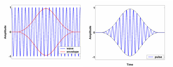
Figure 1. Making a pulse.
In the left hand panel, the two parts of an ultrasonic pulse are shown. The continuous wave is an infinite sine wave, and the red curve is the envelope. The pulse shown in the right hand panel is made by multiplying these two components together. This is the type of pulse we are interested in for this work.
Amazingly ordinary plastic beads
In the region of the ultrasonic spectrum from 1 to 15 MHz water has rather simple properties, exhibiting practically no dispersion. If we place in the water a single plastic sphere with a diameter of about 0.10 mm (roughly the thickness of a human hair), it will efficiently scatter ultrasonic waves in narrow ranges (i.e., bands) of wave frequencies. If we want to make a significant impact on the speed of sound in the water, we have to add in a few thousand of these spheres. The velocity and attenuation data measured from one of these microsphere suspensions is shown in Figure 2. Where a single sphere is an efficient scatterer, a cloud of these spheres strongly attenuate the ultrasonic waves. This attenuation is accompanied by strong dispersion, and it is this dispersion that makes the extreme group velocities for ultrasonic pulses possible. The theory that describes the ultrasonic properties of these water/sphere suspensions has been shown to match very closely to experimental measurements. While recently revisiting the equations for these suspensions, we happened upon the possibility that they could support superluminal group velocities. Surprisingly, the calculations showed that at relatively moderate concentrations of the spheres in water, the group velocity could go beyond c, and even become infinite or negative. After checking the predictions with a more complete form of the theory (accounting for multiple scattering), the results held up. For spheres with an average diameter of 0.1 mm, the calculations showed that a mixture of one part spheres in 20 parts water is enough for the group velocity to reach superluminal values.
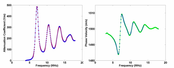
Figure 2. Attenuation and phase velocity data for a microsphere suspension.
The dispersion is the variation is phase velocity. These graphs are from laboratory measurements of 1 part spheres in 100 parts water. The frequencies near 7 MHz, where the main attenuation and dispersion bands occur, are where we focus our attention in this work.
Time is on our side
In order to actually observe a positive superluminal velocity of ultrasound, it would be necessary to control the sphere concentration to an extreme precision. It turns out that the number of spheres required to reach c in our 8 mL sample chamber (a volume a little more than a teaspoon-anda-half) is about 400,000. But the addition of just 4 more beads in the chamber would push it not only beyond c, but beyond infinity into the negative velocity regime. So for these suspensions, going superluminal is practically the same as crossing over to negative velocities. As it turns out, the world of negative velocities is more easily explained in terms of travel times rather than velocity. Velocity is defined as a distance traveled divided by the travel time. To go superluminal means traveling between two points in less time than light does. Negative travel time is a bit puzzling because it implies something reaches a more distant point before it reaches a closer one. This is like throwing a rock at a window and having it appear on the other side before it breaks the glass. It certainly does not fit with our ordinary notions of cause and effect. But pulses of ultrasound are not likes rocks. The key difference is that the rock does not change its size or shape, whereas an ultrasonic pulse does. We can describe the motion of the rock with a single velocity, but assigning a single speed to an ultrasonic pulse in a dispersive medium does not tell the whole story.
Whats with all this negativity?
The main obstacle to understanding negative travel times originates from the mental images we have of a pulse entering and moving through a material. Much like the rock thrown at a window, we picture the pulse traveling through space from shallower to deeper points in the suspension, and can scarcely envision the possibility that its peak somehow gets to deeper points first. It turns out that these mental images are essentially correct, and its our misunderstanding of how the time delay is measured that is the problem. It is important to make a distinction between the peak of the pulse in space at fixed time (i.e., the crest), and the peak of the pulse in time at a fixed depth. To measure the velocity of the peak, imagine putting an ultrasound receiver at different depths along the path of a wave packet (see Figure 3). At each depth, the receiver measures the amplitude of the packet as a function of time as it moves by. By comparing the time it takes the pulse maximum to reach each depth, one can calculate a velocity for the peak. In any material with attenuation, there can be a difference between the positions of the peak as viewed in space (which we will refer to as the crest) versus the peak measured as a function of time at a fixed depth. Its a surprising result but one that is simple to demonstrate. Lets look at the signal captured by our ultrasonic receiver for a simple case where there is no dispersion. What we want to compare is the peak amplitude of the pulse measured as a function of time and the position of the crest of pulse. Here are two animations to help us understand this idea. In Movie 1, there are two panels, one for space and one for time. The top panel shows the bell-shaped pulse envelope propagating through space from left to right (the waves are omitted for clarity). The dotted line in the top panel marks the position of a receiver. The bottom panel shows the signal recorded by the receiver as the envelope passes by. Nothing surprising happens here - the peak in the signal recorded by the receiver coincides with the arrival of the crest of the envelope. In Movie 2 we look at this same experiment in a medium with attenuation. The pulse is attenuated exponentially with depth as it moves deeper. Note that the crest of the pulse is too big to fit in the graph at first, but gets smaller as it moves to the right. In contrast to the previous case, we now see that the peak in the signal shown in the bottom graph occurs well before the crest of the pulse reaches the receiver. The point is that following the pulse envelope as it moves through space can be deceptive because the actual peak we are interested in is hidden in that view. To reliably detect the peak we must monitor the pulse with a receiver and record the amplitude as a function of time. It is this peak in time that we use as our reference point for making velocity measurements. In fact, when dispersion effects are included, a pulse can be so strongly distorted that there may be no readily apparent crest in the space view. But by monitoring the pulse at a fixed depth with a receiver, a peak in time can be clearly defined.
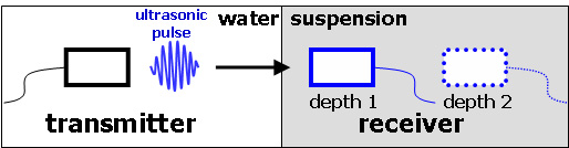
Figure 3. An experimental set-up to measure the group velocity.
An ultrasonic pulse is transmitted into the suspension and the signal is captured by a receiver. The receiver is then moved deeper and the measurement is repeated. The velocity can be determined from the difference in arrival times of the peak at these different depths.
Show me the movie
The distortion in the pulse envelope mentioned above refers to an effect called pulse reshaping. So not only does the pulse peak in time separate from the peak in space, but the pulse gets continually deformed. This reshaping effect also contributes to the superluminal effect. With that in mind, lets look at some simulations of pulse propagation in these microsphere suspensions. As a warm up, well look a case in which the group velocity is normal (i.e., not superluminal). Movie 3 shows an ultrasound pulse propagating in space and time as it enters one of the suspensions from a region of pure water. In this case the concentrations are low (1% spheres by volume), similar to those used in previous laboratory experiments. The pulse is cut-off at the leading and trailing edges, and these slight discontinuities give rise to narrow signals called transients as it moves deeper into the suspension. The transient signals are not as strongly attenuated as the main body of the pulse. So as the pulse propagates we see the main pulse whither away and the transients become the prominent features of the wave packet. In the time record in the bottom panel, we also see that the peak occurs earlier than the passing of the wave crest. Eventually the main pulse is effectively swallowed up by the transients. The strong attenuation is something we have to live with because it accompanies the dispersion effect we need to get superluminal group velocity.
Now we are ready to look at superluminal pulse propagation with negative travel time. Here the experimental set-up as shown in Figure 4 is used. Two identical pulses are fired at the same time, each in line with one of the receivers shown in the figure. The receivers are at different depths in the suspension. As with the previous animations, Movie 4 has the dual view of space and time. In the top panel we now mark the positions of two receivers with colored vertical lines. In the bottom panel, we show the signals recorded by each of the two receivers. The signal from the shallower receiver is colored green, and the signal from the deeper receiver is colored blue. It is the difference in arrival time of the two peaks in the signals in the bottom panel that give us the delay. What the movie shows is that the deeper receiver will detect the peak in its signal before the shallower one, and this is a clear indication of a negative delay time. Notice that in the top panel, the pulse as viewed in space is severely attenuated with depth. The only structures that survive the trip are the transients at the edges, which are like the skeletal remains of the original pulse.
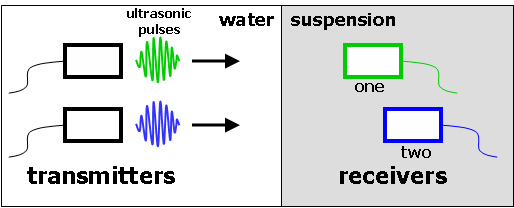
Figure 4. The experimental set-up for the simulations shown in Movies 4 and 5.
Two transmitters emit identical pulses at the same time, and they are captured as signals by receivers which sit at different depths. In Movie 4, the positions of the two receivers are fixed. In Movie 5, one receiver is positioned just inside the suspension and the other is continually moved deeper after each signal is recorded.
The last animation, Movie 5, shows a slightly different experiment, also for a negative travel time. In this movie, we discard the view in space and only look at the signals from the two receivers. For this simulation, one receiver is placed just inside the suspension and the second receiver is put in at a greater depth. Each movie frame shows the two recorded signals from a single experiment (for clarity, only the envelope of the first receivers signal is shown). Between each frame of the movie, the second receiver is moved a little bit deeper into the suspension and the experiment is repeated. In the first part of the movie, the peak recorded by the deeper receiver occurs earlier in time than for the receiver at the surface, clearly exhibiting the negative travel time effect. The peak of the pulse moves forward in time as the receiver goes deeper, but the front edge of the pulse is moving to later times. Eventually, the strong attenuation with depth overwhelms the pulse, and as peak and the front edge approach each other, the original peak gets swept up by the transient. As the receiver goes even deeper, there is no trace of the original pulse and we can no longer see the superluminal effect. Note that the edge transients keep the normal time ordering, that is, they are continually shifting to later times as the receiver moves farther away from the surface. This simulation shows how attenuation limits our ability to measure superluminal effects since beyond a certain depth because the original pulse gets erased from existence.
Now back to the relativity question. As mentioned in the introduction, the key to making sense of superluminal travel lies in paying careful attention to the details. Figure 5 shows a few individual frames from a simulation like that of Movie 5, illustrating the negative delay effect and the limited range over which it is observable. Notice that the earliest parts of the signal from the deeper receiver never occur before the front edge of the surface signal. Any pulse we send out will have some edges, and the pulse envelope will try to outrun those edges - but it is doomed to fail. Although the peak can travel faster-than c, the leading edge of the pulse moves with an ordinary speed of sound. It is this leading edge that really determines how fast you can send a signal, not the peak, because the leading edge always leaves the source first and arrives at the destination first. The pulse envelope, although moving faster, is not able to outrun the waves that support it. So the superluminal pulse inevitably dies out before it can do anything really amazing, like send a signal faster-than-light.
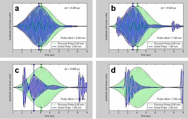
Figure 5. The evolution of superluminal signals.
This figure compares the signals captured by two receivers, one positioned just inside the suspension and the other one at progressively deeper points. The green signal is from the receiver close to the surface. In (a), the peak from the deeper receiver (blue curve) arrives first, signifying the negative travel time of the pulse envelope. In (b), the signal shape remains intact and the deeper receiver records a peak that is even earlier in time than in (a), while the front edge of the signal moves to a later time. In (c), the deeper signal is much more distorted and whats left of the original pulse about to be swept up by the front edge signal. In (d), the original pulse is gone and only the transients from the edges remain.
The sum of it all
Clearly these superluminal ultrasonic waves fit neatly within relativity theory our basic notion of cause and effect. Most scientists (with at least one notable exception) who have studied dispersion-related superluminal propagation would likely agree this phenomenon does not allow faster than light signaling. In any case, there are certainly interesting deeper issues to be explored in the world of superluminal propagation, and perhaps some practical applications may grow out of it (e.g., electronic filters, high frequency oscillators, etc). The fact that the superluminal regime can be explored with ultrasound is surprising, but the established theory clearly says it can.
So, can there be ultrasonic waves that move faster than the speed of light? Our calculations have found that it is not only possible, but well within our means to observe in the lab. Is the recipe for superluminal ultrasound exotic? No, simply take twenty parts water and add one part plastic beads a spoonful of this mixture is all we really need. Is all of this at odds with Professor Einstein? No, a dilute collection of plastic beads might be capable of some unexpectedly remarkable things, but they cant send information faster than light.
Movies
Movie 1. Views of pulse propagation in space and time.
In the top panel, the envelope of a pulse is shown as it moves through space. The dotted line marks the position of a receiver that records the amplitude of the envelope as it moves by. The signal is displayed as a function of time in the bottom panel. In this case, there is no attenuation and the arrival time of the peak in the bottom panel coincides with the passing of the wave crest in the top panel.
Movie 2. Space and time views of pulse propagation with attenuation.
The set-up is the same as Movie 1, except the envelope is attenuated as it moves deeper into the medium. In this case, the peak in the signal is recorded before the crest of the envelope reaches the receiver. This shows that when attenuation is present, the peak in space and the peak amplitude in time are not the same.
Movie 3. Simulation of pulse propagation in a microsphere suspension in the subluminal regime.
The top panel shows the pulse as it propagates in space into the suspension. The black vertical solid line marks the water/suspension boundary. The blue vertical dotted line marks the depth at which a receiver has been placed. The bottom panel shows the signal captured by the receiver as a function of time.
Movie 4. Simulation of pulse propagation in a microsphere suspension in the superluminal regime (space/time split view).
The experimental set-up is shown in Figure 4. The top panel shows the pulse as it propagates in space into the suspension, now at a concentration sufficient to support negative travel times. The two dotted vertical lines mark the depths at which the two respective receivers have been placed. The bottom panel shows the signals captured by the receivers as a function of time. Even though the pulse has to travel farther to reach it, the deeper receiver records the signal peak before the shallower receiver does.
Movie 5. Another simulation of pulse propagation in a microsphere suspension in the superluminal regime (time-only view).
In this simulation, one receiver is fixed just below the surface while the second one is moved deeper into the suspension after each signal capture. Each frame of the movie shows the outputs of the two receivers (the waves in the surface signal are omitted for clarity). Initially, the negative travel time is apparent as the deeper receiver records a peak earlier in time than its partner. Beyond a critical depth, the original pulse is attenuated away and only the transients remain, leaving no trace of the superluminal effect.