Mark Prior – mark.prior@ctbto.org
David Brown
Georgios Haralabus
Mario Zampolli
Preparatory Commission for the Comprehensive Nuclear-test-ban Treaty Organization,
PO Box 1200
1400 Vienna
Austria
Popular version of paper 4pAO1
Presented Thursday afternoon, December 5, 2013
166th ASA Meeting, San Francisco
Devices that listen for underwater sounds generated by nuclear tests can be used to describe the 'soundscape' of noises produced by whales, breaking ice, earthquakes and volcanoes.
The Preparatory Commission for the Comprehensive Nuclear Test Ban Treaty Organization (CTBTO) operates the International Monitoring System (IMS), a worldwide network designed to detect signals caused by nuclear-test explosions. The network has seismometers to detect vibrations in the earth, microphones to listen for very low frequency sounds in the air (infrasound) and radiation sensors that 'smell the air' for radioactive gases and particles produced by nuclear explosions. The IMS also uses underwater microphones (hydrophones) to detect sound in the ocean.
IMS hydrophones are attached to shore stations by cables that can be up to 100 km long. These cables provide power and are connected to a satellite link that sends data to the International Data Centre (IDC) at the CTBTO headquarters in Vienna, Austria. Each cable lies on the seabed and three hydrophones are floated up from it. The hydrophones are arranged in a triangle, 2 km apart at a depth of about 1000 m. This shape allows the arrival time of signals to be measured, along with the direction from which they arrive. Time and direction data are used to calculate the times and locations of the events that produced the signals. Events detected by the IMS network include earthquakes, volcanoes and mining blasts, as well as nuclear-test explosions. Data from the IMS are processed at the IDC 24 hours a day and a list of events is produced for every day of the year.
To understand how well the IMS hydrophone sensors are working, and to help predict how this might change in the future, the CTBTO produces 'soundscapes'. These are descriptions of how the underwater world sounds, in the same way that a 'landscape' is a description of how the earth's surface looks. Two different descriptions are used. The first shows how the strength of sound changes with frequency and time. The second shows the directions from which signals arrive.
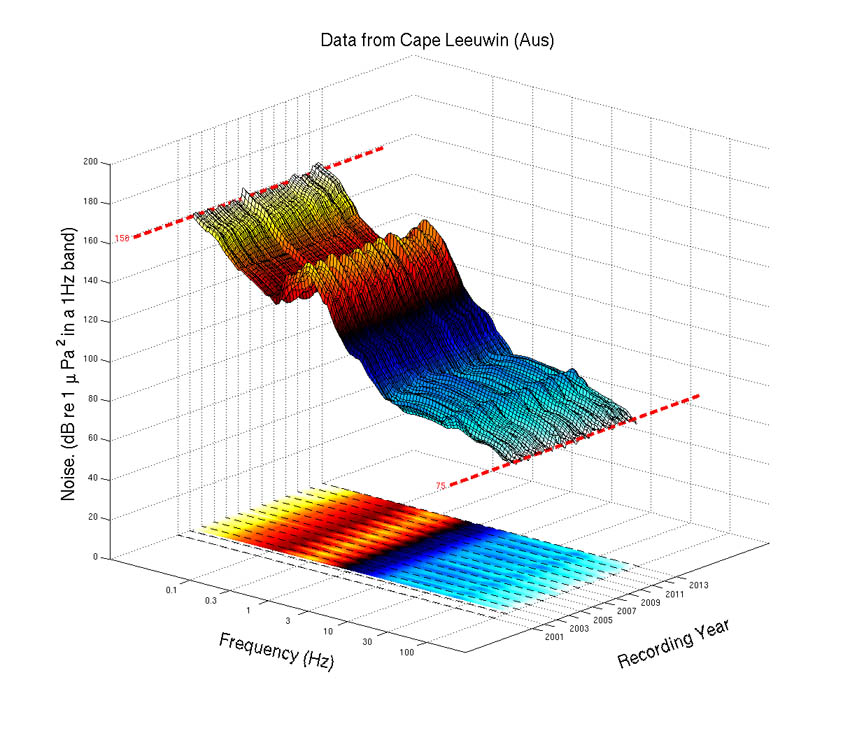
Fig. #1: Soundscape for the IMS hydrophone station off Cape Leeuwin, Western Australia
Fig. 1 shows noise data measured at the Cape Leeuwin IMS station, off the coast of Western Australia. Data are shown for the whole period that the station has been working, with noise levels calculated for frequencies between 0.01 Hz and 100 Hz (human hearing covers an approximate frequency range between 20 Hz and 20,000Hz). The height and colours of the surface in the figure are set by the noise in decibels, relative to one micropascal, which scientists use as the reference value for underwater sound pressure levels. The 'carpet' on the floor of the figure shows the same data 'flattened out' so that only the colour shading is left. This is done because some features in the data are clearer in the flat image, while others show up better on the surface. The underwater noise levels in the figure should not be confused with values quoted for airborne sounds made by rock concerts or jet engines. Different reference levels are used for airborne sounds and the numbers cannot be directly compared.
The ridge in the surface that runs through all years at a frequency of 0.3 Hz is made by sounds produced by water waves on the sea surface. These waves make noises that travel down towards the seabed. The sound waves hit the seafloor and make vibrations in the earth's crust. These vibrations - known as 'the ocean microseism' - are seen even in the middle of continents, thousands of kilometres away from the coast. The bright yellow patches in the 'carpet' in the figure show that the peaks along the ridge happen in the southern-hemisphere winter, when the southern Indian Ocean is roughest.
The surface in Fig. 1 shows small 'hills' at frequencies around 20 Hz in the early months of each year. These hills are caused by whale calls that are heard at Cape Leeuwin during the yearly migration of fin and blue whales.
The data shown in Fig. 1 are useful when working out how sensitive each hydrophone station is. The quietest signal that a station can detect is controlled by the noise in the frequency band containing the signal. The figure shows how this changes as the source of the noises (ice-breaking, whales, storms etc.) changes throughout the year. If underwater noise increased with time, because of more ship traffic for example, this would make the IMS network less sensitive. Data of the sort shown in Fig. 1 are used to look for signs of this happening so that future performance can be predicted.
Although plots like Fig. 1 are very useful, they do not show important information about the direction from which signals arrive. A second, separate plot is used for this and an example is shown in Fig. 2.
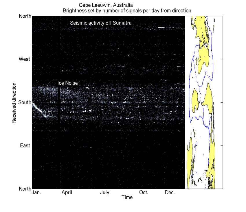
Fig. #2: The directions from which sound arrives at the IMS hydrophone station off Cape Leeuwin, Western Australia
Fig. 2 shows the directions from which signals arrived at the Cape Leeuwin station during the year 2010. For each day, a grey dot is drawn in the figure for 360 directions moving clockwise from north to south then back up to north again. Light-grey or white dots show directions and days on which many arrivals were seen. The map to the right of the figure is a 'Cape Leeuwin's eye view' of the world, where continents are placed according to their direction and distance from the station. The "stretching" according to direction and distance from Cape Leeuwin is responsible for the warped appearance of the map. The blue lines in the map show mid-ocean spreading ridges. These are places where earthquakes are common.
The broad, grey stripe in Fig. 2 shows that signals arrive at Cape Leeuwin from the south all year round. The map region matching this stripe covers Antarctica and this helps to identify ice noise as the source of many of the arrivals. Inside the broad stripe, thinner, brighter lines can be seen. These are caused by single, drifting icebergs that leave Antarctica and move with ocean currents, breaking up as they melt.
The thin, grey line near the top of the figure shows a direction to the northwest of the station from which signals arrive throughout the year. The map shows that this direction points to the coast of Indonesia where there are many earthquakes. These signals are called T-phases and are noises in the ocean made when earthquakes make the coast or underwater mountains shake. Towards the end of the year, Fig. 2 shows a bright line just above the thin stripe. This line begins suddenly then gradually fades from white, through grey to black. This type of feature is made by large earthquakes and the aftershocks that follow them. In this case, the line in Fig. 2 was made by a magnitude 7.7 earthquake on the 25th of October, 2010 off the west coast of Sumatra in Indonesia. This earthquake caused a 3-metre-high tsunami and killed over 400 people. Data from the IMS, including hydrophone stations, are sent to tsunami warning centres around the world and helped to produce a tsunami warning that was sent on the day of the earthquake that caused the line in Fig. 2.
More information about the CTBTO can be found on its website (www.ctbto.org), Facebook page (www.facebook.com/CTBTO) and twitter feed (www.twitter.com/ctbto_alerts). Some examples of the sounds recorded on hydrophone stations are on YouTube under the heading 'CTBTO Sound Quiz'. The views expressed in this paper are those of the authors and do not necessarily represent the views of the CTBTO Preparatory Commission.