1aPAb1 – On the origin of thunder: reconstruction of lightning flashes, statistical analysis and modeling

Arthur Lacroix – arthur.lacroix@dalembert.upmc.fr
Thomas Farges –thomas.farges@cea.fr
CEA, DAM, DIF, Arpajon, France

Régis Marchiano – regis.marchiano@sorbonne-universite.fr
François Coulouvrat – francois.coulouvrat@sorbonne-universite.fr
Institut Jean Le Rond d’Alembert, Sorbonne Université & CNRS, Paris, France

Popular version of paper 1aPAb1
Presented Monday morning, November 5, 2018
176th ASA Meeting, Vancouver, Canada

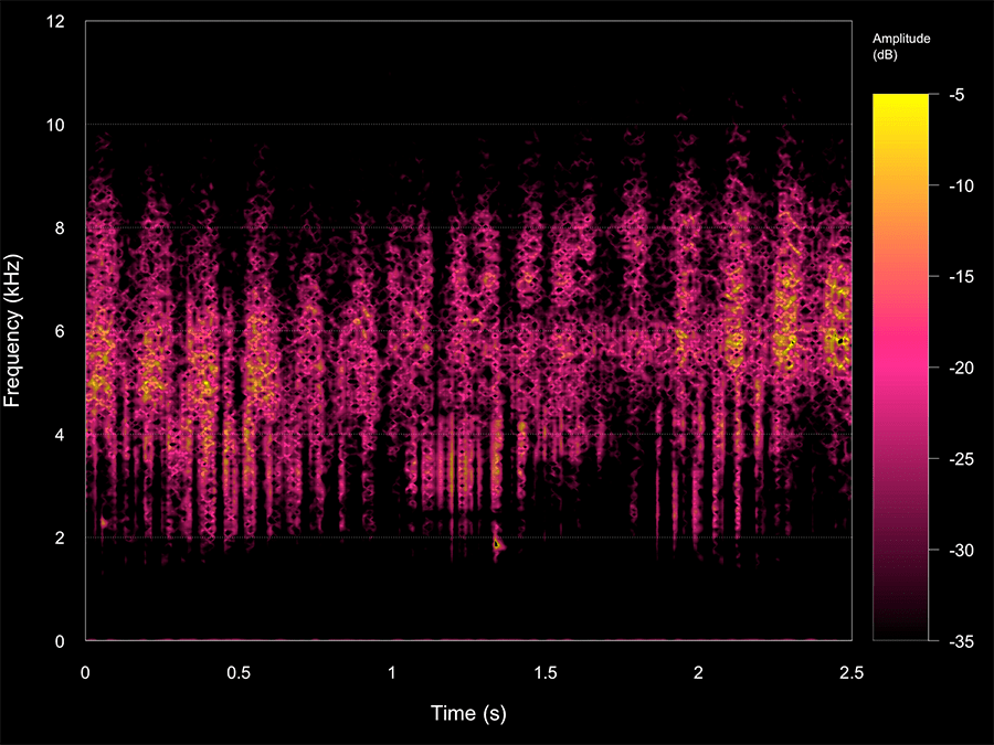
Thunder is the sound produced by lightning, a frequent natural phenomenon occurring in the mean about 25 times per second somewhere on the Earth. The Ancients associated thunder with the voice of deities, though old Greek scientists like Aristotle invoked some natural causes. Modern science established the link between lightning and thunder. Although the sound is audible, thunder also contains an infrasonic frequency component, non-audible by humans, whose origin remains controversial. As part of the European project HyMeX on the hydrological cycle of the Mediterranean region, thunder was recorded continuously by an array of four microphones during two months in 2012 in Southern France, in the frequency range of 0.5 to 180 Hz covering both infrasound and audible sound. In particular, 27 lightning flashes were studied in detail. By measuring the time delays between the different parts of the signals at different microphones, the direction from which thunder comes is determined. Dating the lighting ground impact and therefore the emission time, the detailed position of each noise source within the lightning flash can be reconstructed. This “acoustical lightning photography” process was validated by comparison with a high frequency direct electromagnetic reconstruction based on an array of 12 antennas from New Mexico Tech installed for the first time in Europe. By examining the altitude of the acoustic sources as a function of time, it is possible to distinguish, within the acoustical signal, the part that originates from the lightning flash channel connecting the cloud to the ground, from the part taking place within the ground. In some cases, it is even possible to separate several cloud-to-ground branches. Thunder infrasound comes unambiguously mainly from return strokes linking cloud to ground. Our observations contradict one of the theories proposed for the emission of infrasound by thunder, which links thunder to the release of electrostatic pressure in the cloud. On the contrary, it is in agreement with the theory explaining thunder as resulting from the sudden and intense air compression and heating – typically 20,000 to 30,000 K – within the lightning stroke. The second main result of our observations is the strong dependence of the characteristics of thunder with the distance between the lightning and the observer. Although a common experience, this dependence has not been clearly demonstrated in the past. To consolidate our data, a theoretical model of thunder has been developed. A tortuous shape for the lightning strike between cloud and ground is randomly generated. Each individual part of this strike is modeled as a giant spark, solving the complex equations of hydrodynamics and plasma physics. Summing all contributions, the lightning stroke is transformed into a source of noise which is then propagated down to a virtual listener. This simulated thunder is analyzed and compared to the recordings. Many of our observations are qualitatively recovered by the model. In the future, this model, combined with present and new thunder recordings, could potentially be used as a lightning thermometer, to directly record the large, sudden and yet inaccessible temperature rise within the lightning channel.

acoustical lighting photography

2pSC34 – Distinguishing Dick from Jane: Children’s voices are more difficult to identify than adults’ voices

Natalie Fecher – natalie.fecher@utoronto.ca
Angela Cooper – angela.cooper@utoronto.ca
Elizabeth K. Johnson – elizabeth.johnson@utoronto.ca

University of Toronto
3359 Mississauga Rd.,
Mississauga, Ontario L5G 4K2 CANADA

Popular version of paper 2pSC34
Presented Tuesday afternoon, November 6, 2018, 2:00-5:00 PM, UPPER PAVILION (VCC)
176th ASA Meeting, Victoria, Canada

Parents will tell you that a two-year-old’s birthday party is a chaotic place—young children running around, parents calling out to their children. Amidst that chaos, if you heard a young child calling out, asking to go to the bathroom, would you be able to recognize who’s talking without seeing their face? Perhaps not easily as you might expect, suggests new research from the University of Toronto.

Adults are very adept at recognizing other adults from only their speech. However, children’s speech productions differ substantially from adults, arising from differences in the size of their vocal tracts, to how well they can control their articulators (e.g., tongue) to form speech sounds, to differences in their linguistic knowledge. As a result, a child may pronounce words like elephant and strawberry more like “ephant” and “dobby”. We know very little about how these differences in child and adult speech might affect our ability to recognize who’s talking. Previous work from our lab demonstrated that even mothers are surprisingly not as accurate as you might expect at identifying their own child’s voice.

Sample of 4 adult voices 

4 child voices producing the word ‘elephant’

In this study, we used two tasks to shed light on differences between child and adult voice recognition. First, we presented adult listeners with pairs of either child or adult voices to determine if they could even tell them apart. Results revealed that listeners were substantially worse at differentiating child voices relative to adult voices.

The second task had new adult listeners complete a two-day voice learning experiment, where they were trained to identify a set of 4 child voices on one day and 4 adult voices on the other day. Listeners first heard each voice producing a set of words while seeing a cartoon image on the screen, so they could learn the association between the cartoon and voice. During training, they heard a word and saw a pair of cartoon images, after which, they selected who they thought was speaking and received feedback on their accuracy. Finally, at test, they heard a word and saw 4 cartoon images on the screen and selected who they thought was speaking (Figure 1).

Children’s voices

Figure 1. Paradigm for the voice learning task

Results showed that with training, listeners can learn to identify children’s voices above chance, though child voice learning was still slower and less accurate than adult voice learning. Interestingly, no relationship was found between a listeners’ voice learning performance with adult voices and their voice learning performance with child voices, such that those who were relatively good at identifying adult voices were not necessarily also good at identifying child voices.

This may suggest that the information in the speech signal that we use to differentiate adult voices may not be as informative for identifying child voices. Successful child voice recognition may require re-tuning our perceptual system to pay attention to different cues. For example, it may be more helpful to attend to the fact that one child makes certain pronunciation errors, while another child makes a different set of pronunciation errors.

1pAB1 – Listening to rivers and lakes to help conservation in freshwater environments

Camille Desjonquères1,2,3desjonqu@uwm.edu
Fanny Rybak3, Toby Gifford4, Simon Linke5, Jérôme Sueur2

1 Molecular and Behavioural Ecology Group, Department of Biological sciences, University of Wisconsin-Milwaukee, Milwaukee, United States
2 Muséum national d’Histoire naturelle, Institut Systématique, Evolution, Biodiversité, ISYEB, UMR 7205 CNRS MNHN UPMC EPHE, 45 rue Buffon, 75005 Paris, France
3NeuroPsi, CNRS UMR 9197, Bâtiment 446, Université Paris-Sud, 91405 Orsay cedex, France
4SensiLab, Monash University, Caulfield, VIC 3045, Australia
5Australian Rivers Institute, Griffith University, Nathan, QLD, 4111, Australia

Popular version of paper 1pAB1
Presented Monday afternoon (1:00-1:20 pm), November 5, 2018
176th ASA Meeting, Victoria, Canada

Healthy freshwater environments are essential to the survival of many living organisms including humans. Disturbingly, these environments are so impacted by human activity that biodiversity is declining faster in rivers and lakes than any other type of environment: between 1970 and 2012 populations declined by 81% in freshwater systems compared with 38% and 36% for terrestrial and marine systems respectively (WWF, 2016). Action must be taken to protect these environments, and for this efficient monitoring of ecosystem condition is crucial.

There are several sources of sounds that can be heard underwater in lakes and rivers. Many animals communicate through sound, including frogs, fish (Fig. 1), insects (Fig. 2) and some crustaceans. Water flow and pebbles rolling at the bottom of rivers and streams can be very informative about the physical structure of the environment. The most surprising source of sound may be that of breathing and photosynthesizing plants (Fig. 3).

Figure 1: Video of a pool with spangled grunters (Leiopotherapon unicolor) and juvenile sooty grunters (Hephaestus fuliginosus). Both species are emitting grunts. Recorded in Talaroo (Queensland, Australia).

Effective restoration and protection actions requires detailed knowledge of the environments. It is therefore necessary to survey and monitor freshwater environments. Most current methods used to survey freshwater environments such as netting and electrofishing suffer some limitations: (i) they can injure wildlife, (ii) they only provide a snapshots of the environment, and (iii) they can require a significant workforce. In this presentation, we propose that using sounds recorded underwater with hydrophones is a powerful method to survey freshwater environments.

(Cdesjonqueres_fig2.png and Cdesjonqueres_fig2.wav)

Figure 2: Spectrogram and associated recording of a true bug (Hemiptera) chorus recorded at night in Talaroo (Queensland, Autralia).

The use of sounds recorded in the environment for ecological surveys is studied in the field of ecoacoustics. Ecoacoustic monitoring relies on non-invasive methods that only require the introduction of an acoustic sensor in the environment. Automatic recorders allow for continuous monitoring and reduces the amount of workforce required. Freshwater ecoacoustic monitoring therefore seems like a great complement to more typical surveying methods.

Figure 3: Video of a plant expelling gas bubbles underwater and associated hydrophone recording (Video courtesy of François Vaillant). The legend in the video at 4 seconds reads ‘little bubbles coming out of the leaf’ and at 30 seconds says ‘a ‘big’ bubble is forming at the surface of the leaf’.

Ecoacoustic monitoring is an extremely promising method, already used in terrestrial and marine environments, but that is yet to be operationalized in freshwater environments. Our current research aims at standardizing temporal and spatial sampling designs as well as investigating the links between acoustic and habitat condition in freshwater environments. Overcoming those challenges will allow the application of ecoacoustic monitoring to a broad range of conservation and ecological research questions including the detection of rare or invasive species as well as condition surveys (e.g. polluted vs pristine) or rapid biodiversity assessments.

References:
WWF (2016) Living Planet Report 2016: Risk and Resilience in a New Era. WWF international, Gland, Switzderland.

4aNS11 – Lombard Effect In Restaurant Setting: How Much Would You Spend To Eat At This Restaurant?

Pasquale Bottalico – pb81@illinois.edu

University of Illinois – Department of Speech and Hearing Science
901 South 6th Street
Champaign, IL 61820

Popular version of paper 4aNS11, “Lombard Effect In Restaurant Setting: How Much Would You Spend To Eat At This Restaurant?”
Presented Thursday morning, November 8, 2018, 11:40-12:00 AM, SALON C (VCC)
Joint Meeting 176th ASA Meeting and 2018 Acoustics Week in Canada (CAA), Victoria BC, Canada

This study was conducted to determine the exact point when the noise in a restaurant setting causes vocal discomfort for customers. Another aim of the study was to identify customers’ willingness to spend time and money in a restaurant depending on the varying noise level in the environment.

According to the 2016 Zagat State of American Dining report, 25 percent of restaurant customers consider noise the most irritating component of dining out (Figure 1).

Figure 1. Results from the 2016 National Dining Trends survey of Zagat

The Lombard effect is when speakers unconsciously increase the loudness level of their speech in the presence of background noise in order to be understood. This requires increased vocal effort and can cause vocal fatigue over time. In a restaurant setting particularly, background noise created by other patrons’ conversations is more likely to trigger the Lombard effect than other types of background noise [1] (Figure 2). Previous studies have demonstrated that uncomfortably loud levels of background noise can result in decreased customer satisfaction and business for the restaurant [2, 3].

Figure 2. Example of a noisy restaurant

The Lombard effect has been investigated in a variety of environmental settings with different types and levels of background noise.  However, little is known about the level of background noise that will cause the Lombard effects in restaurant settings.

Fourteen male and 14 female college students with normal hearing were recruited to participate in the study. They read passages to a listener in the presence of typical restaurant noise (as in the attached audio clip) with the level varying between 35 dBA and 85 dBA. Participants were instructed to be sure that the listener could understand them equally well in each condition. (Figure 3)

Lombard Effect

Figure 3. Experimental setup


Restaurant noise

For each noise condition, the participants were then instructed to answer questions about the disturbance they perceived from the noise, how long they would enjoy spending time in this restaurant setting, and how much money they would spend at this restaurant.

The results showed that both participant vocal effort and disturbance increased as the background noise level increased. Reported willingness to spend time and money at a restaurant decreased as the background noise level increased. The participants started to be disturbed at noise levels higher than 52.2 dB(A) (Figure 4, blue line). Because of the disturbance in the communication, participant vocal effort increased at a doubled rate as the background noise level increased (Figure 4, red line) for noise levels higher 57.3 dB(A) (approximately the level of normal conversational speech). Similar noise levels to the one that starts the communication disturbance (51.3 dB(A) and 52.5 dB(A)) also trigger a decrease in the willingness to spend time and money in a restaurant (Figure 4, green and yellow lines). In conclusion, to improve the acoustic environment of restaurants, background noise levels should be lower than 50-55 dB(A). This will minimize the vocal effort of patrons and the disturbance in their communication. Concurrently, this will increase business for the restaurant since patrons would be willing to spend more time and money to eat in a restaurant with a background noise lower than 50-55 dB(A).

Figure 4. Relationship between the level of the noise in dB(A) and self-reported communication disturbance (blue line), relative voice level (red line), willingness to spend time (green line) and willingness to spend money (yellow line), where the error bands indicate the standard error. Vertical dashed lines mark the change-points.

Bibliography
[1]A. Astolfi and M. Filippi, “Good acoustical quality in restaurants: a comparison between speech intelligibility and privacy,” in Proceedings of EuroNoise (2003).

[2] C. C. Novak, J. La Lopa, and R. E. Novak, “Effects of sound pressure levels and sensitivity to noise on mood and behavioral intent in a controlled fine dining restaurant environment,” Journal of Culinary Science & Technology 8(4), 191-218 (2010).

[3] W. O. Olsen, “Average speech levels and spectra in various speaking/listening conditions: A summary of the Pearson, Bennett, & Fidell (1977) report,” American Journal of Audiology 7(2), 21-25 (1998).

1aAB7 – Drum fish spawning doesn’t miss a beat in the eye of a hurricane

Christopher R. Biggs – cbiggs@utexas.edu
Brad Erisman – berisman@utexas.edu

The University of Texas at Austin, Marine Science Institute
750 Channel View Drive,
Port Aransas, TX 78373

Popular version of paper 1aAB7
Presented Monday morning, November 5, 2018
176th ASA Meeting, Victoria, BC

Drum fish

Photo credit: Tyler Loughran

The location and frequency of spawning (reproduction) in fish has a direct effect on the abundance, stability, and resilience of a fish population. Major storm events, such as hurricanes, provide a natural experiment to test the ability of a fish population to withstand disturbances. Acoustic monitoring of Spotted Seatrout spawning revealed that these fish are extremely productive, spawning every day of the spawning season (April – September), including during a category 4 hurricane. These results illustrate the amazing resilience of estuarine fishes to intense disturbances and their potential to cope with projected increases in extreme weather events in the future.

Spotted Seatrout and many other species of “drum fish” make characteristic sounds during spawning (figure 1), which can be heard on underwater microphones, or hydrophones. This allows us to remotely monitor when fish spawn and how long they spawn for, which is especially helpful in murky water, where it is difficult to see. Seatrout spawning can be identified within the audio recordings by analyzing the intensity of the sound within the specific frequency range (250-500 Hz) of the Spotted Seatrout calls.

Figure 1. Recording of male Spotted Seatrout drumming sounds during spawning.

We monitored Spotted Seatrout spawning from April to September 2017 at 15 sites within the estuaries of South Texas, to see how changes in environmental conditions affected spawning. Our study also coincided with a category 4 hurricane. Hurricane Harvey made landfall 9 km east of Rockport, Texas on August 25, 2017 at 17:00 h CST. The eye of the storm was 28 km wide, maximum sustained winds were 59 m s-1 with gusts up to 65 m s-1, and the storm surge caused water levels to rise 3.8 meters above ground level.

The sound pressure level within the frequency range of seatrout spawning sounds peaked every evening between 20:00 and 21:00, indicating that spawning was occurring on a daily basis. During the hurricane wind-associated noise masked any potential spawning sounds, except at two stations that were directly in the path of the hurricane. When the eye of the storm was directly overhead those stations, wind-associated noise decreased, and spawning sounds were audible (figure 2). The time that spawning began shifted two hours earlier for five days after the storm, which may have been partly caused by the decrease in water temperature.

Figure 2. Spectrograms of recordings during Hurricane Harvey showing storm noise at 21:55 and seatrout chorusing at 22:25 within the 250-500 Hz bandwith (dotted lines).

Species that live and spawn in estuaries must deal with conditions that can change rapidly and unpredictably. It is important to understand how those changes impact spawning activity in order to maintain sustainable populations for the fishing industry. Further, understanding how fish respond to environmental disturbances in these environments may offer insight on how fish will respond to climate change and other human impacts elsewhere.

5pAOa7 – Estimating muddy seabed properties using ambient noise coherence

David R. Barclay1– dbarclay@dal.ca
Dieter A. Bevans– dbevans@ucsd.edu
Michael J. Buckingham– mbuckingham@ucsd.edu

  1. Department of Oceanography, Dalhousie University, 1355 Oxford St, Halifax, Nova Scotia, B3H 4R2, CANADA
  2. Marine Physical Lab, Scripps Institution of Oceanography, University of California, San Diego, 9500 Gilman Drive, #0238, La Jolla CA, 92093-0238

Popular version of paper 5pAOa7: “Estimating muddy seabed properties using ambient noise coherence”
Presented Friday afternoon, November 9th, 2018, 3:00 – 3:15PM, Esquimalt Room 176th ASA Meeting, Victoria, B.C.

Figure 1. The autonomous Deep Sound acoustic recorder on the rear deck of the R/V Neil Armstrong

The ocean is a natural acoustic waveguide, bounded by the sea surface and seabed, inside which sound can travel large distances. In the frequency range of 10’s – 1000’s of Hertz, seawater is nearly transparent to sound, absorbing only a small fraction of energy of the acoustic wave as it propagates in the ocean. However, sound transmitted in this shallow water ocean waveguide reflects off the bottom, losing some energy which is either transmitted into the bottom, or absorbed by the sediment. In order to predict and model the distances over which any acoustic ocean monitoring, detection, or communication systems may operate, accurate knowledge of the acoustic properties (the sound speed, attenuation, and density) of the seabed must be known.

The majority of the ocean’s bottom has a top layer of sand or gravel, where the grain sizes are large enough that gravity and friction dictate the micro-physics at inter-granular contacts and play a large roll in determining the sound speed and attenuation in the material. In silts and clays (a.k.a. muds), grain sizes are on the order of microns or less, so electrochemical forces become the dominant factor responsible for the mechanics of the medium. Mud particles are usually elongated, with high length-to-width ratios, and when consolidated they form stacks of parallel grains and ‘card-house’ structures, giving the ensemble mechanical and acoustical properties unlike larger grained sands.

In March and April 2017, as part of the ONR-supported Seabed Characterization Experiment (SCE) designed to investigate the geo-acoustic properties of fine-grained sediments, a bottom lander known as Deep Sound was deployed on the New England Mud Patch (NEMP) from the R/V Neil Armstrong. The NEMP occupies an area of approximately 13,000 kmoff the east coast of the USA, 95 km south of Martha’s Vineyard, and is 170 km wide, descending 75 km across the continental shelf with an unusually smooth bathymetry. The region is characterized by a layer of mud, accumulated over the last 10,000 years, estimated to be as thick as 13 meters [1].

seabed

Figure 2. Location of the five Deep Sound deployments, plotted over the two-way travel time, a proxy for mud layer thickness (where 16 milliseconds is equivalent to 13 meters)

Drop #1

Drop #2

Drop #3

Drop #4

Drop #5

Two way travel time [ms]

The American naturalist Louis François de Pourtalès first described this ocean feature in 1872 [2], in the context of a convenient navigation aid for whaling ships headed into Nantucket and New Bedford. Sailors would make depth soundings using a lead weight with a plug of wax on the bottom which collected a small sample of the seabed. Since the mud bottom was unique along the New England seaboard, ships were able to determine their location in relation to their home ports in foggy weather.

Deep Sound (Fig. 1) is a free-falling (untethered), four channel acoustic recorder designed to descend from the ocean’s surface to a pre-assigned depth, or until pre-assigned conditions are met, at which point it drops an iron weight and returns to the surface under its own buoyancy with a speed of ~0.5 m/s in either direction. In this case, the instrument was configured to land on the seabed, with the hydrophones arranged in an inverted ‘T’ shape, and continue recording until either a timer expired, or a battery charge threshold was crossed. Almost 30 hours of ambient noise data were collected at five locations on the NEMP, shown in Fig. 2.

From the vertical coherence of the ambient noise, information about the geo-acoustic properties of the seabed was extracted by fitting the data to a model of ocean noise, based on an infinite sheet of sources, representing the bubbles generated by breaking ocean surface waves. The inversion returned estimates of five geo-acoustic properties of the bottom: the sound speed and attenuation, the shear-wave speed and attenuation, and the density of the muddy seabed.


  1. Bothner, M. H., Spiker, E. C., Johnson, P. P., Rendigs, R. R., Aruscavage, P. J. (1981). Geochemical evidence for modern sediment accumulation on the continental shelf off southern New England. Journal of Sedimentary Research, 51(1), pp. 281-292.
  2. Pourtales, L.F., (1872). The characteristics of the Atlantic sea bottom off the coast of the United States: Report, Superintendent U.S. Coast Survey for 1869, Appendix 11, pp. 220-225.
  3. Carbone, N. M., Deane, G. B., Buckingham, M. J., (1998). Estimating the compressional and shear wave speeds of a shallow water seabed from the vertical coherence of ambient noise in the water column. The Journal of the Acoustical Society of America, 103(2), pp. 801-813.